Geometrical orbitals

Orbital geometry for 2 (rotating) mass points;

${\displaystyle n_{g}={\frac {n_{p}}{\sqrt {N}}}}$ (pixel to mass ratio)

${\displaystyle d={\sqrt {2\alpha }}{\frac {n_{p}}{\sqrt {N}}}=({\sqrt {2\alpha }})n_{g}}$ (pixel aggregate)

${\displaystyle r=2\alpha n_{p}^{2}=d^{2}N}$ (orbital length)

Hyper-sphere co-ordinates

A relativistic hyper-sphere expands in uniform incremental steps (the simulation clock-rate) at the speed of light, and so time and velocity are constants. Particles are pulled along by this expansion, the expansion as the origin of motion, and so all objects, including orbiting objects, travel at, and only at, the speed of light in these hyper-sphere co-ordinates ^[3]. Time becomes time-line.

B's orbit relative to A's time-line axis in time units t

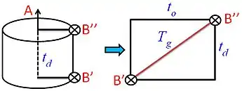
While B (satellite) has a circular orbit period t_o on a 2-axis plane (horizontal axis as 3-D space) around A (planet), it also follows a cylindrical orbit (from B¹ to B¹¹) around the A time-line axis in hyper-sphere co-ordinates (vertical axis). A is moving with the universe expansion (along the time-line) at (v = c) but is stationary in 3-D space (v = 0). B is orbiting A at (v = c) but the time-line axis motion is equivalent (and so `invisible') to both A and B and so from the perspective of A, the period of 1 B orbit along the observable 2-axis plane = T_g at velocity (${\displaystyle v=2\pi r/T_{g}}$) and for B the orbital period = t_d.

We can simplify this cylinder by projecting it onto a 2-axis plane as the difference between 2 orbits.

${\displaystyle t_{small}=2\pi {\frac {dN}{2}}}$

${\displaystyle t_{large}=2\pi d^{3}N}$

${\displaystyle t=t_{large}-t_{small}=2\pi (d^{3}-{\frac {d}{2}})N}$

${\displaystyle v={\frac {2\pi r}{t}}={\frac {d}{d^{2}-{\frac {1}{2}}}}}$

We place 2 point mass on opposite poles on a circular ring forming a gravitational orbital pair. For each unit of time, the ring rotates, the degree of rotation according to the ring radius. In the simulations depicted here the rotation is anti-clockwise. An orbital of minimum radius would have an orbital period t_p measured in base time units with angle of increment β

${\displaystyle t_{p}=2\pi (d^{3}-{\frac {d}{2}})=28456.6547...;\;n_{g}=1}$

${\displaystyle \beta ={\frac {1}{(d^{3}-{\frac {d}{2}})}}}$

In orbits with multiple points, N>1. Example: a 4-body (4-point) orbit comprising 1-point (r = 13623) orbiting a 3-point center (see 4-body orbit diagram). The 3 center points (centered 0, 0) are then repeated to simulate increasing mass (λ_orbit = 2N, kr = 28456.6547....)

Each of the 6 orbiting pairs are calculated independently. All results are then summed and averaged before the next unit of time is incremented. Thus the universe simulation can be updated in real-time on a serial processor.

8-body (8 mass points, 27 orbitals) orbit

Planck units

The above can also be measured in terms of the dimensioned Planck units. As ${\displaystyle n_{g}}$ can therefore be used as a measure of length to mass, when ${\displaystyle n_{g}}$ =1, N = ${\displaystyle n_{p}^{2}}$ and so between objects A and B (where mass M_A >> m_B), 2Nl_p = λ_A.

λ_object = Schwarzschild radius

m_P = Planck mass

l_p = Planck length

${\displaystyle N_{points}={\frac {M_{A}}{m_{P}}}}$ (number of particles in the Planck mass point-state per unit of Planck time)

${\displaystyle r_{g}=d^{2}N_{points}l_{p}=\alpha n_{g}^{2}\lambda _{A}}$ (converting to Schwarschild radius)

${\displaystyle v_{g}={\frac {c}{d}}}$ (gravitational orbit velocity)

${\displaystyle T_{g}={\frac {2\pi r_{g}}{v_{g}}}}$ (standard gravitational orbit period)

${\displaystyle a_{g}={\frac {v_{g}^{2}}{r_{g}}}}$ (gravitational acceleration)

Hyper-sphere orbital

Measuring a hypersphere orbital along a 2-D plane in 3-D space

${\displaystyle t_{o}={\frac {2\pi r_{g}}{c}}}$

${\displaystyle t_{d}=T_{g}{\sqrt {1-{\frac {v_{g}^{2}}{c^{2}}}}}={\sqrt {T_{g}^{2}-t_{o}^{2}}}=t_{o}{\sqrt {{2\alpha n_{g}^{2}}-1}}=t_{o}{\sqrt {d^{2}-1}}}$

If we consider the smaller orbit as a rotation of the orbital plane itself (for both orbits, orbital velocity = c) then we can re-write the above as;

${\displaystyle t_{plane}=2\pi {\frac {dN}{2}}{\frac {l_{p}}{c}}}$

${\displaystyle T_{g}=2\pi d^{3}N{\frac {l_{p}}{c}}}$

${\displaystyle t_{d}=T_{g}-t_{plane}=2\pi (d^{3}-{\frac {d}{2}})N{\frac {l_{p}}{c}}}$

${\displaystyle v_{plane}={\frac {c}{2d^{3}}}}$

${\displaystyle t_{d}={\frac {2\pi r_{g}}{(v_{g}+v_{plane})}}}$

Example: B orbital period at r = 42164.170 km (n = 5889.674)

${\displaystyle t_{plane}=.453x10^{-5}}$ s

${\displaystyle v_{plane}=.1617x10^{-6}}$ m/s

${\displaystyle v_{g}=3074.66}$ m/s

T_g = 86164.0916523 s

t_d = 86164.0916478 s

By including the rotation of the orbital plane, B only requires t_d time units to complete 1 orbit in hyper-sphere co-ordinates.

Precession

The ellipticity of the B orbit around A.

semi-minor axis: ${\displaystyle b=\alpha l^{2}\lambda _{A}}$

semi-major axis: ${\displaystyle a=\alpha n^{2}\lambda _{A}}$

radius of curvature :${\displaystyle L={\frac {b^{2}}{a}}={\frac {al^{4}\lambda _{A}}{n^{2}}}}$

${\displaystyle {\frac {3\lambda _{A}}{2L}}={\frac {3n^{2}}{2\alpha l^{4}}}}$

arc secs per 100 years:

${\displaystyle 1296000{\frac {3n^{2}}{2\alpha l^{4}}}{\frac {100T_{earth}}{T_{planet}}}}$

Mercury = 42.98  
Venus = 8.62  
Earth = 3.84  
Mars = 1.35  
Jupiter = 0.06

The orbital plane becomes

${\displaystyle t_{plane}=2\pi ({\sqrt {2\alpha }})^{5}nl^{4}N_{sun}{\frac {l_{p}}{3c}}}$

Mercury

${\displaystyle t_{plane}{\frac {42.98}{1296000}}=100*365.245*24*3600}$s

Examples

i) Earth orbits

${\displaystyle N_{points}={\frac {M_{earth}}{m_{P}}}}$

Earth surface orbit

rg = 6371.0 km  
ag = 9.820m/s^2
Tg = 5060.837s
vg = 7909.792m/s

Geosynchronous orbit

rg = 42164.0km   
ag = 0.2242m/s^2
Tg = 86163.6s
vg = 3074.666m/s

Moon orbit (d = 84600s)

rg = 384400km   
ag = .0026976m/s^2
Tg = 27.4519d
vg = 1.0183km/s

ii) Planetary orbits

${\displaystyle N_{points}={\frac {M_{sun}}{m_{P}}}}$

mercury: rg = 57909000km, Tg = 87.969d, vg = 47.872km/s 
venus: rg = 108208000km, Tg = 224.698d, vg = 35.020km/s 
earth: rg = 149600000km, Tg = 365.26d, vg = 29.784km/s 
mars: rg = 227939200km, Tg = 686.97d, vg = 24.129km/s 
jupiter: rg = 778.57e9m, Tg = 4336.7d, vg = 13.056km/s
pluto: rg = 5.90638e12m, Tg = 90613.4d, vg = 4.740km/s 

iii) The energy required to lift a 1 kg satellite into geosynchronous orbit is the difference between the energy of each of the 2 orbits (geosynchronous and earth).

${\displaystyle E_{orbital}={\frac {hc}{2\pi r_{6371}}}-{\frac {hc}{2\pi r_{42164}}}=0.412x10^{-32}J}$

${\displaystyle N_{links}={\frac {M_{earth}m_{satellite}}{m_{P}^{2}}}=0.126x10^{41}}$

${\displaystyle E_{total}=E_{orbital}N_{links}=53MJ/kg}$

Angular momentum

The orbital angular momentum of the planets derives from the angular momentum of the orbital pairs (and so is independent of the orbital angular momentum of the sun).

${\displaystyle N_{sun}={\frac {M_{sun}}{m_{P}}}}$

${\displaystyle N_{planet}={\frac {M_{planet}}{m_{P}}}}$

${\displaystyle N_{links}=N_{sun}N_{planet}}$

mercury = .9153 x1039  
venus    = .1844 x1041  
earth    = .2662 x1041 
mars     = .3530 x1040 
jupiter   = .1929 x1044   
pluto   = .365 x1039   

Rotational angular momentum

${\displaystyle N_{links}=(N_{planet})^{2}}$

The rotational angular momentum ${\displaystyle L_{ram}}$ contribution to planet rotation.

${\displaystyle v_{rot}={\sqrt {N_{points}}}{\frac {c}{2\alpha n_{p}}}={\frac {c}{2\alpha n_{rot}}}}$

${\displaystyle T_{rot}={\frac {2\pi r}{v_{rot}}}}$

${\displaystyle L_{ram}={\frac {2}{5}}{\frac {2\pi Mr^{2}}{T}}=({\frac {2}{5}})N_{links}\;n_{rot}{\frac {h}{2\pi }},\;{\frac {kgm^{2}}{s}}}$

Earth:

T_rot = 83847.7s (86400)

v_rot = 477.8m/s (463.3)

${\displaystyle L_{ram}=.727\;x10^{34}\;{\frac {kgm^{2}}{s}}}$ (.705)

Mars:

T_rot = 99208s (88643)

v_rot = 214.7m/s (240.29)

${\displaystyle L_{ram}=.187\;x10^{33}{\frac {kgm^{2}}{s}}\;}$(.209)

Rotational angular momentum combined with v_rot

${\displaystyle L_{ram}v_{rot}=({\frac {2}{5}})N_{links}{\frac {hc}{2\pi 2\alpha }},\;{\frac {kgm^{3}}{s^{2}}}}$

8-body (8 mass points, 27 orbitals) orbit

Wave-state

To illustrate how this might apply, I use best fit geometries t_p for H and P orbitals (n = 1). The electron orbits with the orbital plane (H example) and against the orbital plane (P example).

${\displaystyle v_{a}={\frac {c}{2\alpha n}}}$

${\displaystyle r_{a}=\alpha n^{2}(\lambda _{orbital})}$

H (1s-2s) transition = 2466061413 MHz ^[4].

${\displaystyle \lambda _{e}=.3861592676\$e-12m}$

${\displaystyle \lambda _{p}=.2103089101\$e-15m}$ ^[5]

${\displaystyle T_{a}=2\pi {\frac {\alpha (\lambda _{e}+\lambda _{p})}{v_{a}}}}$

${\displaystyle t_{p}={\frac {4{\sqrt {3}}}{{\sqrt {\alpha }}^{3}}}}$

${\displaystyle t_{o}=T_{a}t_{p}}$

${\displaystyle t_{d}=T_{a}{\sqrt {1-t_{p}^{2}}}={\sqrt {T_{a}^{2}-t_{o}^{2}}}=t_{o}{\sqrt {1/t_{p}^{2}-1}}}$

${\displaystyle {\frac {3}{4t_{d}}}=2466061423\;MHz}$

Positronium (1s-2s)= 1233607216 MHz ^[6]

${\displaystyle T_{a}=2\pi {\frac {\alpha (2\lambda _{e})}{v_{a}}}}$

${\displaystyle t_{p}={\frac {56}{3{\sqrt {\alpha }}^{3}}}}$

${\displaystyle t_{d}=T_{a}{\sqrt {1+t_{p}^{2}}}={\sqrt {T_{a}^{2}+t_{o}^{2}}}=t_{o}{\sqrt {1/t_{p}^{2}+1}}}$

${\displaystyle {\frac {3}{4t_{d}}}=1233607221\;MHz}$

Orbital transition

Atomic electron transition is the change of an electron from one energy level to another. The following redefines the Rydberg formula in terms of `physical' orbitals, where transition is an orbital replacement, the electron plays no pre-dominant role.

Consider the Hydrogen Rydberg formula for transition between and initial ${\displaystyle i}$ and a final ${\displaystyle f}$ orbit. The incoming photon ${\displaystyle \lambda _{R}}$ causes the electron to `jump' from the ${\displaystyle n=i}$ to ${\displaystyle n=f}$ orbit.

${\displaystyle \lambda _{R}=R.({\frac {1}{n_{i}^{2}}}-{\frac {1}{n_{f}^{2}}})={\frac {R}{n_{i}^{2}}}-{\frac {R}{n_{f}^{2}}}}$

The above could be interpreted as referring to 2 photons;

${\displaystyle \lambda _{R}=(+\lambda _{i})-(+\lambda _{f})}$

Let us suppose a region of space between a free proton ${\displaystyle p^{+}}$ and a free electron ${\displaystyle e^{-}}$ which we may define as zero. This region then divides into 2 waves of inverse phase which we may designate as photon (${\displaystyle +\lambda }$) and anti-photon (${\displaystyle -\lambda }$) whereby

${\displaystyle \lambda _{R}=(+\lambda _{i})-(+\lambda _{f})}$

The photon (${\displaystyle +\lambda }$) leaves (at the speed of light), the anti-photon (${\displaystyle -\lambda }$) however is trapped between the electron and proton and forms a standing wave orbital. Due to the loss of the photon, the energy of (${\displaystyle p^{+}+e^{-}+-\lambda )<(p^{+}+e^{-}>+0}$) and so stable.

Let us define an (${\displaystyle n=i}$) orbital as (${\displaystyle -\lambda _{i}}$). The incoming Rydberg photon ${\displaystyle {\lambda _{R}}=(+\lambda _{i})-(+\lambda _{f})}$ arrives in a 2-step process. First the ${\displaystyle (+\lambda _{i})}$ adds to the existing (${\displaystyle -\lambda _{i}}$) orbital.

${\displaystyle (-\lambda _{i})+(+\lambda _{i})=zero}$

The (${\displaystyle -\lambda _{i}}$) orbital is canceled and we revert to the free electron and free proton; ${\displaystyle p^{+}+e^{-}+0}$ (ionization). However we still have the remaining ${\displaystyle -(+\lambda _{f})}$ from the Rydberg formula.

${\displaystyle 0-(+\lambda _{f})=(-\lambda _{f})}$

From this wave addition followed by subtraction we have replaced the ${\displaystyle n=i}$ orbital with an ${\displaystyle n=f}$ orbital. The electron has not moved (there was no transition from an ${\displaystyle n_{i}}$ to ${\displaystyle n_{f}}$ orbital), however the electron region (boundary) is now determined by the new ${\displaystyle n=f}$ orbital ${\displaystyle (-\lambda _{f})}$.

References

- ↑ Macleod, Malcolm J.; "Programming gravity for Planck unit Simulation Hypothesis modeling". RG. Feb 2011. doi:10.13140/RG.2.2.11496.93445/7.
- ↑ Macleod, M.J. "Programming Planck units from a mathematical electron; a Simulation Hypothesis". Eur. Phys. J. Plus 113: 278. 22 March 2018. doi:10.1140/epjp/i2018-12094-x.
- ↑ Macleod, Malcolm J.; "Programming relativity for Planck unit Simulation Hypothesis modeling". RG. Feb 2011. doi:10.13140/RG.2.2.18574.00326/2.
- ↑ Parthey CG et al, {Improved measurement of the hydrogen 1S-2S transition frequency}, Phys Rev Lett. 2011 Nov 11;107(20):203001. Epub 2011 Nov 11
- ↑ M. S. Fee et al., Phys. Rev. Lett. 70, 1397 (1993)