Return to Main Page *Boundary Value Problems

These lessons are to introduce you to Numerical Methods used to calculate numerical solutions to the 2-D BVPs discussed earlier. Two resources that would be useful for the exercises are

1. MATLAB MathWorks
2. MAPLE MAPLE

However any computational system that can solve a system of equations will meet the needs of many of the elementary exercises. Three Linux based packages (free) are:

1. Scilab Scilab (similar to Matlab)
2. Maxima Computer Algebra System Maxima
3. Octave

'

Finite Difference Method

The Finite Difference method is a numerical method used for approximating the solution to a differential equation. The fundamentals of FD methods with application to an ODE and the 1-D heat equation can be found at [Finite Difference: http://en.wikipedia.org/wiki/Finite_difference_method]

A particular application is the Finite Difference Time Domain method to wave propagation problems

Finite Elements Method

The Finite Elements Method constitutes a numerical approach to approximating the solution of an ordinary differential equation over a two-dimensional grid that is not rectangular, or one in which the data points, or nodes, are not evenly spaced. This gives it an advantage over the Finite Differences Method.

The first step of the method consists of triangulating the region to be integrated by dividing it into triangles, with the nodes as vertices. The next step is to determine the values of the unknown function at the nodes. Here is where the "finite elements" come in. A finite element is a function ${\displaystyle \phi _{j}}$ whose graph is a pyramid with its peak over a node ${\displaystyle v_{j}}$. A finite element solution to an ODE is a linear combination of finite elements: ${\displaystyle U(v_{j})=\sum _{j=1}^{n}C_{j}\phi _{j}(v_{j})}$ where ${\displaystyle \phi _{j}(v_{j})={\begin{cases}1{\text{ at j-node}}\\0{\text{ at other nodes}}\end{cases}}}$. The constants ${\displaystyle C_{j}}$ are then the values of the function at the nodes. Once these values are found, each triangle is integrated using the "Three Corners" method (the triangular version of the Trapezoid method) and summed. ^[2]

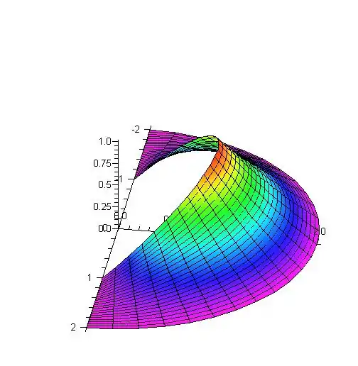
Plot of Finite Difference Example

Example of ${\displaystyle u_{rr}+{\frac {1}{r}}u_{r}+{\frac {1}{r^{2}}}u_{\theta \theta }=0}$ on a half annulus geometry with:

• ${\displaystyle u(1,\theta )=sin(\theta )}$
• ${\displaystyle u(2,\theta )=0}$
• ${\displaystyle u(r,0)=0}$ for ${\displaystyle 1<r<2}$
• ${\displaystyle u(r,\pi )=0}$ for ${\displaystyle 1<r<2}$

]

1. ↑ Boundary Value Problems,Powers 5th edition,Elsevier Academic Press
2. ↑ T. Young and M. Mohlenkamp, Numerical Methods and Matlab Programming For Engineers