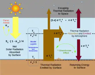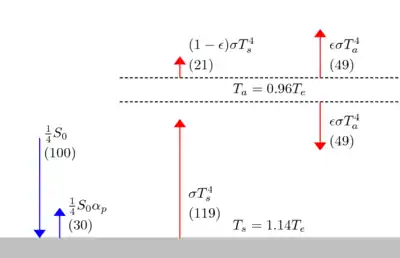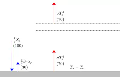
The temperatures of a planet's surface and atmosphere are governed by a delicate balancing of their energy flows. The idealized greenhouse model is based on the fact that certain gases in the Earth's atmosphere, including carbon dioxide and water vapour, are transparent to the high-frequency solar radiation, but are much more opaque to the lower frequency infrared radiation leaving Earth's surface. Thus heat is easily let in, but is partially trapped by these gases as it tries to leave. Rather than get hotter and hotter, Kirchhoff's law of thermal radiation says that the gases of the atmosphere also have to re-emit the infrared energy that they absorb, and they do so, also at long infrared wavelengths, both upwards into space as well as downwards back towards the Earth's surface. In the long-term, the planet's thermal inertia is surmounted and a new thermal equilibrium is reached when all energy arriving on the planet is leaving again at the same rate. In this steady-state model, the greenhouse gases cause the surface of the planet to be warmer than it would be without them, in order for a balanced amount of heat energy to finally be radiated out into space from the top of the atmosphere.[1]
Essential features of this model where first published by Svante Arrhenius in 1896.[2] It has since become a common introductory "textbook model" of the radiative heat transfer physics underlying Earth's energy balance and the greenhouse effect.[3][4][5] The planet is idealized by the model as being functionally "layered" with regard to a sequence of simplified energy flows, but dimensionless (i.e. a zero-dimensional model) in terms of its mathematical space.[6] The layers include a surface with constant temperature Ts and an atmospheric layer with constant temperature Ta. For diagrammatic clarity, a gap can be depicted between the atmosphere and the surface. Alternatively, Ts could be interpreted as a temperature representative of the surface and the lower atmosphere, and Ta could be interpreted as the temperature of the upper atmosphere, also called the skin temperature. In order to justify that Ta and Ts remain constant over the planet, strong oceanic and atmospheric currents can be imagined to provide plentiful lateral mixing. Furthermore, the temperatures are understood to be multi-decadal averages such that any daily or seasonal cycles are insignificant.
Simplified energy flows
The model will find the values of Ts and Ta that will allow the outgoing radiative power, escaping the top of the atmosphere, to be equal to the absorbed radiative power of sunlight. When applied to a planet like Earth, the outgoing radiation will be longwave and the sunlight will be shortwave. These two streams of radiation will have distinct emission and absorption characteristics. In the idealized model, we assume the atmosphere is completely transparent to sunlight. The planetary albedo αP is the fraction of the incoming solar flux that is reflected back to space (since the atmosphere is assumed totally transparent to solar radiation, it does not matter whether this albedo is imagined to be caused by reflection at the surface of the planet or at the top of the atmosphere or a mixture). The flux density of the incoming solar radiation is specified by the solar constant S0. For application to planet Earth, appropriate values are S0=1366 W m−2 and αP=0.30. Accounting for the fact that the surface area of a sphere is 4 times the area of its intercept (its shadow), the average incoming radiation is S0/4.
For longwave radiation, the surface of the Earth is assumed to have an emissivity of 1 (i.e. it is a black body in the infrared, which is realistic). The surface emits a radiative flux density F according to the Stefan–Boltzmann law:
where σ is the Stefan–Boltzmann constant. A key to understanding the greenhouse effect is Kirchhoff's law of thermal radiation. At any given wavelength the absorptivity of the atmosphere will be equal to the emissivity. Radiation from the surface could be in a slightly different portion of the infrared spectrum than the radiation emitted by the atmosphere. The model assumes that the average emissivity (absorptivity) is identical for either of these streams of infrared radiation, as they interact with the atmosphere. Thus, for longwave radiation, one symbol ε denotes both the emissivity and absorptivity of the atmosphere, for any stream of infrared radiation.


The infrared flux density out of the top of the atmosphere is computed as:
In the last term, ε represents the fraction of upward longwave radiation from the surface that is absorbed, the absorptivity of the atmosphere. In the first term on the right, ε is the emissivity of the atmosphere, the adjustment of the Stefan–Boltzmann law to account for the fact that the atmosphere is not optically thick. Thus ε plays the role of neatly blending, or averaging, the two streams of radiation in the calculation of the outward flux density.
The energy balance solution
Zero net radiation leaving the top of the atmosphere requires:
Zero net radiation entering the surface requires:
Energy equilibrium of the atmosphere can be either derived from the two above equilibrium conditions, or independently deduced:
Note the important factor of 2, resulting from the fact that the atmosphere radiates both upward and downward. Thus the ratio of Ta to Ts is independent of ε:
Thus Ta can be expressed in terms of Ts, and a solution is obtained for Ts in terms of the model input parameters:
or
The solution can also be expressed in terms of the effective emission temperature Te, which is the temperature that characterizes the outgoing infrared flux density F, as if the radiator were a perfect radiator obeying F=σTe4. This is easy to conceptualize in the context of the model. Te is also the solution for Ts, for the case of ε=0, or no atmosphere:
With the definition of Te:
For a perfect greenhouse, with no radiation escaping from the surface, or ε=1:
Application to Earth
Using the parameters defined above to be appropriate for Earth,
For ε=1:
For ε=0.78,
- .
This value of Ts happens to be close to the published 287.2 K of the average global "surface temperature" based on measurements.[7] ε=0.78 implies 22% of the surface radiation escapes directly to space, consistent with the statement of 15% to 30% escaping in the greenhouse effect.
The radiative forcing for doubling carbon dioxide is 3.71 W m−2, in a simple parameterization. This is also the value endorsed by the IPCC. From the equation for ,
Using the values of Ts and Ta for ε=0.78 allows for = -3.71 W m−2 with Δε=.019. Thus a change of ε from 0.78 to 0.80 is consistent with the radiative forcing from a doubling of carbon dioxide. For ε=0.80,
Thus this model predicts a global warming of ΔTs = 1.2 K for a doubling of carbon dioxide. A typical prediction from a GCM is 3 K surface warming, primarily because the GCM allows for positive feedback, notably from increased water vapor. A simple surrogate for including this feedback process is to posit an additional increase of Δε=.02, for a total Δε=.04, to approximate the effect of the increase in water vapor that would be associated with an increase in temperature. This idealized model then predicts a global warming of ΔTs = 2.4 K for a doubling of carbon dioxide, roughly consistent with the IPCC.
Tabular summary with K, C, and F units
| ε | Ts (K) | Ts (C) | Ts (F) |
|---|---|---|---|
| 0 | 254.8 | -18.3 | -1 |
| 0.78 | 288.3 | 15.2 | 59 |
| 0.80 | 289.5 | 16.4 | 61 |
| 0.82 | 290.7 | 17.6 | 64 |
| 1 | 303.0 | 29.9 | 86 |
Extensions
The one-level atmospheric model can be readily extended to a multiple-layer atmosphere.[8][9] In this case the equations for the temperatures become a series of coupled equations. These simple energy-balance models always predict a decreasing temperature away from the surface, and all levels increase in temperature as "greenhouse gases are added". Neither of these effects are fully realistic: in the real atmosphere temperatures increase above the tropopause, and temperatures in that layer are predicted (and observed) to decrease as GHG's are added.[10] This is directly related to the non-greyness of the real atmosphere.
An interactive version of a model with 2 atmospheric layers, and which accounts for convection, is available online.[11]
See also
References
- ↑ "What is the Greenhouse Effect?" (PDF). Intergovernmental Panel on Climate Change. 2007.
- ↑ Svante Arrhenius (1896). "On the influence of carbonic acid in the air upon the temperature of the ground". Philosophical Magazine and Journal of Science. 41 (251): 237–276. doi:10.1080/14786449608620846.
- ↑ Marshall J., Plumb R.A., Atmosphere, Ocean and Climate Dynamics, AP 2007, Chapter 2, The global energy balance
- ↑ "ACS Climate Science Toolkit - How Atmospheric Warming Works". American Chemical Society. Retrieved 2 October 2022.
- ↑ "METEO 469: From Meteorology to Mitigation - Understanding Global Warming - Lesson 5 - Modelling of the Climate System". Penn State College of Mineral and Earth Sciences - Department of Meteorology and Atmospheric Sciences. Retrieved 2 October 2022.
- ↑ Kleeman, Richard. "Zero Dimensional Energy Balance Model". math.nyu.edu.
- ↑ Jones, P. D.; New, M.; Parker, D. E.; Martin, S.; Rigor, I. G. (1999). "Surface air temperature and its changes over the past 150 years". Reviews of Geophysics. 37 (2): 173–199. Bibcode:1999RvGeo..37..173J. doi:10.1029/1999RG900002.
- ↑ "ACS Climate Science Toolkit - Atmospheric Warming - A Multi-Layer Atmosphere Model". American Chemical Society. Retrieved 2 October 2022.
- ↑ "Energy Recirculation and a Layered Radiative Atmosphere Model". Climate Puzzles. Retrieved 1 June 2023.
- ↑ Manabe, Syukuro; Wetherald, Richard T. (1 May 1967). "Thermal Equilibrium of the Atmosphere with a Given Distribution of Relative Humidity". Journal of the Atmospheric Sciences. 24 (3): 241–259. Bibcode:1967JAtS...24..241M. doi:10.1175/1520-0469(1967)024<0241:TEOTAW>2.0.CO;2.
- ↑ "2-Layer Atmosphere with Solar, Longwave, & Convection". Denning Research Group, Colorado State University. Retrieved 1 June 2023.
Additional bibliography
- Bohren, Craig F.; Clothiaux, Eugene E. (2006). "1.6 Emissivity and Global Warming". Fundamentals of Atmospheric Radiation. Chichester: John Wiley & Sons. pp. 31–41. ISBN 978-3-527-40503-9.
- Petty, Grant W. (2006). "6.4.3 Simple Radiative Models of the Atmosphere". A First Course in Atmospheric Radiation (2nd ed.). Madison, Wisconsin: Sundog Pub. pp. 139–143. ISBN 978-0-9729033-1-8.