Subject classification: this is a chemistry resource.

Type classification: this is a lesson resource.

A harmonic oscillator (quantum or classical) is a particle in a potential energy well given by V(x)=½kx². k is called the force constant. It can be seen as the motion of a small mass attached to a string, or a particle oscillating in a well shaped as a parabola. This is a very important model because most potential energies can be approximated as parabolas near their minima, and the model allows us to understand the vibrations in molecular systems.

The classical harmonic oscillator

The classical harmonic oscillator is often studied in elementary physics. The solution of Newton's equation gives x(t) = A sin(ωt + φ) (Eq. 1) where ${\displaystyle \omega ={\sqrt {\frac {k}{m}}}}$ is the angular frequency (Eq. 2), A is the amplitude of the motion and φ is its phase.

The total energy does not depend on time.
${\displaystyle E_{tot}=E_{kinetic}+E_{potential}={\frac {1}{2}}m\left({\frac {dx}{dt}}\right)^{2}+{\frac {1}{2}}kx^{2}}$ (Eq. 3) ${\displaystyle E_{tot}={\frac {1}{2}}mA^{2}\omega ^{2}\cos ^{2}\left(\omega t+\varphi \right)+{\frac {1}{2}}mA^{2}\omega ^{2}\sin ^{2}\left(\omega t+\varphi \right)={\frac {1}{2}}m\omega ^{2}A^{2}}$

E_tot is proportional to the square of the amplitude and can be any positive number.

The quantum harmonic oscillator

To find the eigenvalues and eigenfunction of the quantum harmonic oscillator you should solve the following problem: ${\displaystyle \left\{-{\frac {\hbar ^{2}}{2m}}{\frac {\partial ^{2}}{\partial x^{2}}}+{\frac {1}{2}}kx^{2}\right\}\psi (x)=E\psi (x)}$ (Eq. 4)

In this case, the solution will be given without proof. The eigenvalues of the harmonic oscillator are: E_v = ħω(½ + v) where v=0,1,2,... (Eq. 5)

The vibrational quantum number is indicated by v and can take any integer starting from zero. ω is the same angular frequency used for the classical oscillator.

To express the eigenfunctions in a simpler form it is convenient to divide Equation 4 by ħω which gives ${\displaystyle \left\{-{\frac {\hbar }{2m\omega }}{\frac {\partial ^{2}}{\partial x^{2}}}+{\frac {1}{2}}{\frac {m\omega x^{2}}{\hbar }}\right\}\psi (x)={\frac {E}{\hbar \omega }}\psi (x)}$ (Eq. 6)

And by defining a new adimensional variable ${\displaystyle y={\sqrt {\frac {m\omega }{\hbar }}}x}$, the equation takes a very simple form (the same for all oscillators): ${\displaystyle \left\{-{\frac {1}{2}}{\frac {\partial ^{2}}{\partial y^{2}}}+{\frac {1}{2}}y^{2}\right\}\psi (y)={\frac {E}{\hbar \omega }}\psi (y)}$ (Eq. 7)

This is just done to give the eigenfunctions a simpler form. The first four eigenfunctions of the harmonic oscillator Hamiltonian are:

• ${\displaystyle \psi _{0}(y)=N_{0}\exp \left(-{\frac {y^{2}}{2}}\right)}$ (Eq. 8)
• ${\displaystyle \psi _{1}(y)=N_{1}y\exp \left(-{\frac {y^{2}}{2}}\right)}$
• ${\displaystyle \psi _{2}(y)=N_{2}(2y^{2}-1)\exp \left(-{\frac {y^{2}}{2}}\right)}$
• ${\displaystyle \psi _{3}(y)=N_{3}(2y^{3}-3y)\exp \left(-{\frac {y^{2}}{2}}\right)}$

N are just normalization constants. The general structure of the harmonic oscillator wavefunction is: ${\displaystyle \psi (y)=N_{v}H_{v}(y)\exp \left(-{\frac {y^{2}}{2}}\right)}$ (Eq. 9)

In other words, they are the product of a Gaussian function and a polynomial H_v(y) (known by mathematicians as Hermite polynomials and are given in tables for consultation).

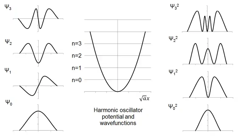
Note that, as in the case of the particle in the box, the number of nodes increases with increasing quantum number and energy.

However, unlike the classical harmonic oscillator, not only are there discrete levels but the ground state does not have zero energy, rather a finite amount (½ħω). This minimal amount of energy is known as the zero point energy.

Tunnelling in classically forbidden region

From the wavefunction ψ_v(x) you can calculate the probability of finding a particle at a given point by taking the modulus squared |ψ_v(x)|². Consider for example the normalized probability density for the ground state. A classical oscillator with the same energy E_v=0=½ħω would oscillate between two turning points -x_T and +x_T where ${\displaystyle x_{T}={\sqrt {\frac {\hbar }{m\omega }}}}$. But the quantum oscillator has some probability of being found at x<-x_T and x>x_T in the classically forbidden region. A particle can be in the classically forbidden region only if it is allowed to have negative kinetic energy, which is impossible in classical mechanics. The phenomenon of quantum particles being able to be in regions of space forbidden to the classical particle is called quantum mechanical tunnelling.

The correspondence principle

We have been listing phenomena (tunnelling, nodal plane, discrete levels of energy) which make quantum mechanic behaviour very different than classical behaviour. Why does classical physics seem to work fine for macroscopic objects? The answer is complicated but a good starting point is the correspondence principle: at very high quantum numbers and energies, the quantum mechanical behaviour coincides with the classical behaviour.

When we observe a macroscopic oscillator, it could be described quantum mechanically but the quantum number would be enormous (see Exercise). If the correspondence principle is correct the quantum and classical probability of finding a particle in a particular position should approach each other for very high energies. This is what happens (question 10).

Exercise Calculate the 3 lowest energy levels of a particle with mass m=1.7x10-24 kg in a one dimensional harmonic potential V(x)=½kx². Use k=100 N/m. The vibration of a diatomic molecule A-B can be approximated as the motion of a harmonic oscillator with potential V(x)=½kx². x in this case represents the displacement from equilibrium distance. Instead of the mass, you have to use the reduced mass μ related to the mass of A and the mass of B: ${\displaystyle \mu ={\frac {m_{A}m_{B}}{m_{A}+m_{B}}}}$. Calculate the vibrational energy ħω of the H2 molecule for which k=510 N/m. Draw the probability density of the first 5 levels of the harmonic oscillator and the first 5 levels of the particle in the box. Compare them. Consider the harmonic oscillator Schrödinger equation written in the adimensional coordinate y as ${\displaystyle \left\{-{\frac {1}{2}}{\frac {\partial ^{2}}{\partial y^{2}}}+{\frac {1}{2}}y^{2}\right\}\psi (y)={\frac {E}{\hbar \omega }}\psi (y)}$. Show that ${\displaystyle \psi _{0}(y)=\exp \left(-{\frac {y^{2}}{2}}\right)}$ and ${\displaystyle \psi _{1}(y)=y\exp \left(-{\frac {y^{2}}{2}}\right)}$ are eigenfunctions of H(y) and find the corresponding eigenvalues. Find the values of x where it is most likely to find a particle in the first excited state of a harmonic oscillator. Show that the classical turning point, xT for an oscillator with energy Ev = (½ + v)ħω is ${\displaystyle x_{T}={\sqrt {\frac {2\left({\begin{matrix}{\frac {1}{2}}\end{matrix}}+v\right)\hbar }{m\omega }}}}$. What is the classically forbidden region? What integral should be solved to find the probability of finding a quantum oscillator in the classically forbidden region? (You don't need to solve the integral.) The harmonic oscillator wavefunctions have the following property: ${\displaystyle y\psi _{v}(y)={\sqrt {v}}\psi _{v-1}(y)+{\sqrt {v+1}}\psi _{v+1}(y)}$ i.e. by multiplying ψv(y) by y gives a linear combination of ψv-1(y) and ψv+1(y). Prove that this is true for v=1 (you should include the normalization constant). Is there a zero point energy for the particle in the box? free particle? A macroscopic pendulum has ω=1 s-1, m=1 kg and total energy 0.1 J. What would be its quantum number if described quantum mechanically? The classical probability of finding an oscillator at one particular position is proportional to its inverse velocity. Why? Show that the classical velocity as a function of the position is ${\displaystyle \omega {\sqrt {x_{T}^{2}-x^{2}}}}$ and the probability density is therefore proportional to ${\displaystyle {\frac {1}{\sqrt {x_{T}^{2}-x^{2}}}}}$. Solutions 1 2 3 We need to show that ${\displaystyle \left\{-{\begin{matrix}{\frac {1}{2}}\end{matrix}}{\frac {\partial ^{2}}{\partial y^{2}}}+{\begin{matrix}{\frac {1}{2}}\end{matrix}}y^{2}\right\}\psi _{0}(y)=E\psi _{0}(y)}$ where ${\displaystyle \psi _{0}(y)=\exp \left(-{\frac {y^{2}}{2}}\right)}$. Substitution gives: ${\displaystyle {\begin{matrix}\left\{-{\begin{matrix}{\frac {1}{2}}\end{matrix}}{\frac {\partial ^{2}}{\partial y^{2}}}+{\begin{matrix}{\frac {1}{2}}\end{matrix}}y^{2}\right\}\exp \left(-{\frac {y^{2}}{2}}\right)=-{\begin{matrix}{\frac {1}{2}}\end{matrix}}{\frac {\partial ^{2}}{\partial y^{2}}}\exp \left(-{\frac {y^{2}}{2}}\right)+{\begin{matrix}{\frac {1}{2}}\end{matrix}}y^{2}\exp \left(-{\frac {y^{2}}{2}}\right)\\=-{\begin{matrix}{\frac {1}{2}}\end{matrix}}{\frac {\partial }{\partial y}}\left(-y\exp \left(-{\frac {y^{2}}{2}}\right)\right)+{\begin{matrix}{\frac {1}{2}}\end{matrix}}y^{2}\exp \left(-{\frac {y^{2}}{2}}\right)\\=-{\begin{matrix}{\frac {1}{2}}\end{matrix}}\left(-\exp \left(-{\frac {y^{2}}{2}}\right)+y^{2}\exp \left(-{\frac {y^{2}}{2}}\right)\right)+{\begin{matrix}{\frac {1}{2}}\end{matrix}}y^{2}\exp \left(-{\frac {y^{2}}{2}}\right)={\begin{matrix}{\frac {1}{2}}\end{matrix}}\exp \left(-{\frac {y^{2}}{2}}\right)\end{matrix}}}$ Comparison of the first and last term confirms that ${\displaystyle \left\{-{\begin{matrix}{\frac {1}{2}}\end{matrix}}{\frac {\partial ^{2}}{\partial y^{2}}}+{\begin{matrix}{\frac {1}{2}}\end{matrix}}y^{2}\right\}\psi _{0}(y)=E\psi _{0}(y)}$ where E = ½. The probability density is proportional to |ψ1(y)|² = y2 exp(-y2) = P (P is the probability). This is maximum or minimum when dP/dy=0. The derivative is ${\displaystyle {\frac {dP}{dy}}=2y\exp(-y^{2})-2y^{3}\exp(-y^{2})=2y\exp(-y^{2})(1-y^{2})}$. This is zero for y=0 (where there is a minimum) and y=±1 (where the two maxima are). The maximum displacement (turning point) of a classical oscillator is when the potential energy ½kxT2 = ½mω2xT2 is equal to the total energy. We get, for E = (½ + v)ħω, (½ + v)ħω = ½mω2xT2 and therefore ${\displaystyle x_{T}={\sqrt {\frac {2\left({\begin{matrix}{\frac {1}{2}}\end{matrix}}+v\right)\hbar }{m\omega }}}}$. The classical region is xT < x < -xT. The probability of being outside this region, i.e. in the interval between -∞ < x < -xT and xT < x < +∞ is ${\displaystyle \int _{-\infty }^{-x_{T}}\psi _{v}(x)^{*}\psi _{v}(x)\,dx+\int _{x_{T}}^{+\infty }\psi _{v}(x)^{*}\psi _{v}(x)\,dx}$. Substituting v=1 in ${\displaystyle y\psi _{v}(y)={\sqrt {\frac {v}{2}}}\psi _{v-1}(y)+{\sqrt {\frac {v+1}{2}}}\psi _{v+1}(y)}$. Left and right hand side are equal, i.e. ${\displaystyle y\psi _{1}(y)={\frac {\sqrt {2}}{\pi ^{1/4}}}y^{2}\exp \left(-{\frac {y^{2}}{2}}\right)}$ so you get ${\displaystyle {\sqrt {\begin{matrix}{\frac {1}{2}}\end{matrix}}}\psi _{0}(y)+{\sqrt {\begin{matrix}{\frac {2}{2}}\end{matrix}}}\psi _{2}(y)={\frac {1}{\pi ^{1/4}}}\left[{\frac {\sqrt {2}}{2}}\exp \left(-{\frac {y^{2}}{2}}\right)+{\frac {\sqrt {2}}{2}}(2y^{2}-1)\exp \left(-{\frac {y^{2}}{2}}\right)\right]={\frac {\sqrt {2}}{\pi ^{1/4}}}y^{2}\exp \left({\frac {y^{2}}{2}}\right)}$. Yes. No, quantization derives from the boundary condition. Without boundaries, there is no quantization and E=0 is allowed. Ev = (½ + v)ħω → v = Ev ÷ ħω - ½ = 0.2 ÷ (1.05x10-34 x 1) - ½ ≈ 1.90x1033 (i.e. very large). You are more likely to observe a particle in a position where it moves slowly. (Think - does a rollercoaster spend more time on the top or at the bottom of its track?) The total energy is Etotal = Ekinetic + Epotential = ½mv2 + ½kx2 and it must be constant. The velocity at a given position x is therefore v = [2/m (Etotal - ½kx2)]1/2. When the particle is at the turning point xT, the velocity is zero so Etotal = 0 + ½kxT2 and the velocity can be written as v = [2/m (½kxT2 - ½kx2)]1/2 = [k/m]1/2(xT2 - x2)1/2 = ω(xT2 - x2)1/2.

Next: Lesson 5 - Further Particles in the Box and Polar Coordinates