< MATLAB

Shown below are the 15 terms of the series for ε equal to 0, .001, and .01, respectively. The series converges to -1/12 in the limit that ε>0 vanishes.
S(ε=.000) = 1.0 + 2.0 + 3.0 + 4.0 + 5.0 + 6.0 + 7.0 + 8.0 + 9.0 + 10.0 + 11.0 + 12.0 + 13.0 + 14.0 + 15.0 + ...
S(ε=.001) = 1.0 + 2.0 + 3.0 + 4.0 + 5.0 + 6.0 + 7.0 + 7.9 + 8.9 + 09.9 + 10.9 + 11.9 + 12.8 + 13.8 + 14.8 + ...
S(ε=.010) = 1.0 + 2.0 + 2.9 + 3.8 + 4.8 + 5.6 + 6.5 + 7.4 + 8.2 + 09.0 + 09.8 + 10.6 + 11.3 + 12.1 + 12.8 + ...

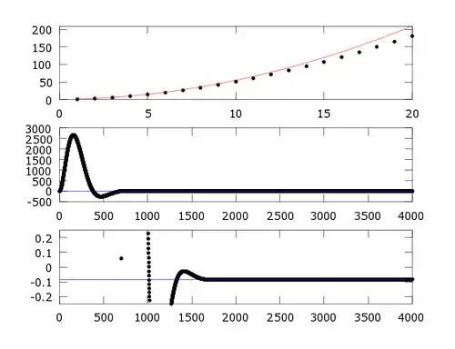
Real part of plotted for n = 1 to 4000 and ε=0.01.
Top: The red line shows that the first 20 of the terms are reasonable approximations to the series 1+2+3+4+...
Middle: After 100 terms, the contributions to the sum become negative and the sum begins to approach zero.
Bottom: By n= 4000 the series has converged to a value very close to -1/12.
Top: The red line shows that the first 20 of the terms are reasonable approximations to the series 1+2+3+4+...
Middle: After 100 terms, the contributions to the sum become negative and the sum begins to approach zero.
Bottom: By n= 4000 the series has converged to a value very close to -1/12.
This code runs on both MATLAB and Octave. It sums,
- where, .
The numerical simulation suggests that for real :
Warning: This result does not hold if is a complex number that goes to zero, unless the real and imaginary parts are constrained to be equal in magnitude. This would be a significant simulation if the series converges to -1/12 for all ratios of real to imaginary parts of ε. Nevertheless, it is curious that a real to imaginary ratio of one yields the well known value, 1/12≈.083333
Questions
- Verify that if ε > 0
- Why is this interesting?
- Can Octave do symbolic integration?
See also
|
|
Output of MATLAB code
The code that follows gave this output:
If z=
0.990000332+0.009900333i the sum from 1 to 4000 of n*z^n is
 -8.333333332e-02 + i 4.999999999e+03
MATLAB/Octave code
% This code is designed to investigate the "astonishing" claim that
%
% 1 + 2 + 3 + 4 + 5 + ... = -1/12
%
% It numerically calculates
%
%   1*z + 2*z^2 + 3*z^3 + 4*z^4 + 5*z^5 + ... N*z^N
%
% where N is large and z is nearly equal to, 1.0 + 0.0i
clear;clc; close all;% clear memory and command window
N=4000; % sets the number of terms in the expansion
shortN=20; % how far we plot to show initial behaviour of the series
alpha=.01; %the real part of z
beta=.01;
epsilon = -alpha+1*i*beta;
% The result is astonishing if alpha=beta
z=exp(epsilon);
theta=atan(abs(imag(z)/real(z)));%is the argument of z
period=round(2*pi/theta);
%We estimate the limit as N->infty by averaging over one period
n=1:N; % the partial sums shall be plotted against these integers
seq=linspace(0,0,N);  % preallocate elements of the sequence {1,2,3...,N}
parsum=linspace(0,0,N);% preallocate the partial sums: {1, 1+2, 1+2+3, ...}
seq(1)=1*z;  % first element of sequence
parsum(1)=seq(1); % first partial sum
%All the partial sums are stored in parsum, all the terms in seq
for count=2:N
    seq(count)=count*z^count;
    parsum(count)=parsum(count-1)+seq(count);
end
parsumR=real(parsum); % we plot only the real part
subplot(3,1,1)
plot(n,parsumR,'.k',[0, N],[-1/12,-1/12],'MarkerSize',6.0,'Linewidth',1.5);
axis([0,shortN,0,shortN*(shortN+1)/2]);
%title('(a) The initial partial sums proceed almost as 1+2+3+4+...');
% The titles do not print properly on Octave and had to be commented out
%plots the first terms (should go as n*(n+1)/2) Verify with parabola:
hold on;
plot(n,n.*(n+1)/2,'-r',[0, N],[-1/12,-1/12]);
hold off;
subplot(3,1,2)
plot(n,parsumR,'.k',[0, N],[-1/12,-1/12],'MarkerSize',8.0);
%title('(b) The small deviation from z=1 introduces decay and oscillation'); %plots all N terms
subplot(3,1,3)
plot(n,parsumR,'.k',[0, N],[-1/12,-1/12],'MarkerSize',8.0);
axis([0,N,-.25,.25]);
%title('(c) The last terms show convergence to approximately -1/12'); %plots the partial sums for the largest values of n.
final=parsum(N);
fprintf('If z= \n%11.9f+%11.9fi ',real(z),imag(z) );
fprintf('the sum from 1 to %d of n*z^n is \n',N );
fprintf(' %11.9e + i %11.9e\n',real(final),imag(final));%this works
%%%%Save the real part of the sequence
for count=1:N
    Rseq(count)=real(seq(count));
end
This article is issued from Wikiversity. The text is licensed under Creative Commons - Attribution - Sharealike. Additional terms may apply for the media files.