Because some curves are too complex to express as a single Bézier curve, a new type of curve is needed. Splines can serve that purpose.
Definition
Historically, shipbuilders would use flexible strips of wood called "splines" placed between metal weights called "ducks". Generally, the curves that were created in this manner were infinitely continuous except at the ducks, where the splines were generally only C0 with each other. B-spline curves, or basis spline curves, are shapes that consists of several Bézier curves. The best way to think of a spline is a machine that generates Bézier curves. An n-degree B-spline curve produces n-degree Bézier curves that are automatically Cn-1 with each other. The advantage to B-splines is that we can represent m Bézier curves of degree n with m+n B-spline control points, far less than the nm+1 control points that a string of Bézier curves requires.
The following explanation of B-splines is not a "traditional" explanation. B-splines contain a lot of intense mathematics and most of the algorithms aren't intuitive. This explanation will attempt to show the mechanism behind B-splines. From here, an explanation of the recurrence relations and mathematics that can be found other places on the Web will make more sense. This will not be a cursory explanation; even though this tutorial will be simple to understand, the techniques shown here are powerful and can be implemented computationally if desired.
Polar Form of B-spline Points
Dr. Lyle Ramshaw introduced a powerful notation for B-spline control points: the polar form. It is a powerful tool that allows B-splines to be described simply. There are 4 rules for the polar labels (the labels for the control points):
- For an n-degree Bézier curve P[a,b](t), we must label each control point with a polar label. The new label for the point , where:
- Thus, for a degree-3 Bézier curve, the polar labels become P0 = P(a,a,a), P1 = P(a,a,b), P2 = P(a,b,b), P3 = P(b,b,b).
- A B-spline with a knot vector has polar labels that follow the relation.
- For a knot vector [0,1,2,3,4,5] of a degree 3 B-spline, then P0 = P(0,1,2), P1= (1,2,3), P2= (2,3,4), P3= (3,4,5).
- The arguments of a polar label are symmetric. It means that they can be changed in any order and still maintain the description of the point.
- Example: P(0,2,5,4) = P(4,2,0,5) = P(2,4,5,0), etc.
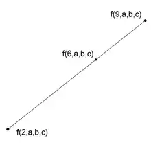
- Polar labels with only one different argument lie on the same line.
- In the example at the right, the polar labels only differ by 1 number. A point can be found by interpolating the line, just as the polar label f(6,a,b,c) can be found by interpolating between the points labeled f(2,a,b,c) and f(9,a,b,c). The point is located 3/7 of the distance from f(2,a,b,c) and f(9,a,b,c). The general equation is given for f(u1,u2,...,un-1,a), f(u1,u2,...,u_n-1,b), f(u1,u2,...,un-1,c):
- As you can see, it's the same formula as for the affine transformation of a line.
The Knot Vector
The knot vector is simply a collection of parameter values for the individual Bézier curves that make up a B-spline. For example, if we have a cubic B-spline and want to spline together a series of Bézier curves with intervals of [2,3], [3,5], [5,6], and [6,9], the knot vector would be . The knots in the vector must be arranged in an ascending order. There can be repeated knots values, for example, the knot vector [0,1,2,3,3,3,4,5,5,6] is perfectly valid. Repeated knots do affect the curve, however. You might have noticed the other knots appended to the knot vector. There are always n-1 knots appended to the front and back of the knot vector. These knots specify the end conditions of the B-spline. For example, if t0 = t1 = 2, then the endpoint of the B-spline with parameter values [2,3] will pass through the endpoint of the B-spline. This will also be the case at the other endpoint if 9 = t7 = t8.
Most representations of the knot vector require n end condition knots. This is mainly just a historical convention. In the above example, if we added knots to either end to make 3 end condition knots since n = 3 (i.e. ), they wouldn't affect the curve at all. It does appear a lot in other B-spline discussions, so I make it point to mention it here.
Sometimes we talk about the spacing of a knot vector, or the difference between successive knot values. If a knot vector is evenly spaced, like [0,1,2,3,4,5,6], then we call it a uniform B-spline. If the knot vector is unevenly spaced, then we call it a non-uniform B-spline.
Generation of Bézier Curves
If the B-splines are just a way to generate Bézier curves, where are the Bézier curves? Well, we have B-spline control points, but we need a way to get the Bézier control points. This is where the polar labels come in. We have to establish the rules for assigning polar labels to B-spline control points.
For a degree-n curve, we take the first n knots in the knot vector and load them into the polar label for the first control point. For the second control point, we take n knots again, but we take the 2nd knot to the (n+1)th knot. We repeat this process until we go through the whole knot vector. For example, if we have a cubic B-spline with a knot vector [0,0,0,1,3,5,7,7,7], we get the following labels for the B-spline:
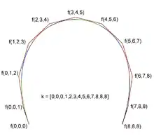
The picture at right shows the Bézier curves that the B-spline curve generated. If we remember how polar labels describe Bézier curves, a degree 3 Bézier curve with an interval from [a,b] has polar labels f(a,a,a), f(a,a,b), f(a,b,b), f(b,b,b). In the pictured example, we know the 1st Bézier curve has parameter values from [0,1]. To fully describe this curve, we would need points with polar labels f(0,0,0), f(0,0,1), f(0,1,1), f(1,1,1). As we can see, the curve has the first 2 polar labels, but not f(0,1,1) and f(1,1,1). How do we get them? We can use the 4th rule of polar labels. We know that f(0,1,1) is 1/2 the distance from f(0,0,1) and f(0,1,2), so we can label a point there. We can find f(1,1,2) by the same method. Then, we can see that f(1,1,1) is halfway between f(0,1,1) and f(1,1,2). Now we have all the control points that describe the Bézier curve. It's that simple. We can use this technique to generate the Bézier curves from any B-spline.
Knot Vector Insertion
In a sense, we've already covered knot insertion. Knot insertion is when a value is inserted into the knot vector. So what happens when we insert a knot? Let's start with a simple degree-3 B-spline, [0,0,0,1,2,2,2]. The polar labels for this curve are f(0,0,0), f(0,0,1), f(0,1,2), f(1,2,2), and f(2,2,2). If we inserted a 1 in the knot vector, the vector would become [0,0,0,1,1,2,2,2]. This would change the polar labels that describe the points for the curve:
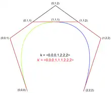
Inserting another 1 in the knot vector would just give us the point f(1,1,1). The knot vector in this case would be [0,0,0,1,1,1,2,2,2]. We can see that we get the control points for all the Bézier curves that describe the B-spline. When we were generating the Bézier curves in the section above, we were interpolating the points. In that example, we had the points f(0,0,0) and f(0,0,1) and we were solving for the points f(0,1,1) and f(1,1,1). We would have gotten the same results we calculated for if the knot vector had been [0,0,0,1,1,1,2,3,4,5,6,7,8,8,8]. So we know that by inserting repeated knots, we can get the control points for the constituent Bézier curves. In this example, we saw that we "traded" the point f(0,1,2) for the two points f(0,1,1) and f(1,1,2) by inserting the 1 into the knot vector. So what happens if the knot value we insert is not a repeat? For the vector [0,0,0,1,3,3,3], inserting a 2 would change the polar labels like so:
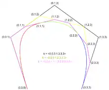
Here, we simply "traded" the 2 points f(0,1,3) and f(1,3,3) for the 3 points f(0,1,2), f(1,2,3), and f(2,3,3).
Repeating knot insertion on a degree-n B-spline until there are n repeated knots is a technique to evaluate the B-spline at any parameter value. This is called the the de Boor algorithm. De Boor's algorithm is analogous to de Casteljau's algorithm for Bézier curves; in fact, it's a generalization of de Casteljau's algorithm.
Multiple Knots
If the same knot value appears in the knot vector more than once, we call it a multiple knot. We can say at that point, there is a degenerate Bézier curve that has parameter values from [t,t], where t is the repeated knot value. Now let's talk about continuity. In general, a degree-n B-spline automatically generates Bézier curves that are Cn-1 continuous. We can see that the degree-3 B-spline in the pictured example has Bézier curves that look C2. However, this is only the case only when there are no multiple knots. We know the curves in the example are C2 because no knot value is repeated. However, if the knot vector was [0,0,0,1,1,2,3,4,5,6,7,8,8,8], then the continuity is no longer C2 between every curve. At t=1, the Bézier curves would be only C1 at that point because of the repeated knot. Remember that at t=0 and t=8, we have end conditions. It could be said that because we have a triple knot at the ends, the ends of the B-spline are only C0.
Periodic B-splines
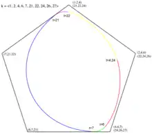
A special case of the B-spline is a periodic B-spline. This is simply a B-spline that ends where it begins, making a closed loop. In the image at right, each of the Bézier curves that is generated by the B-spline is colored. But how was this curve generated? There are only 2 constraints on a B-spline curve that must be met in order to turn it into a periodic B-spline. As shown, the knot vector has 10 knots in it. A cubic B-spline curve with 10 knots must have 8 control points, but where are the other three? The first 3 control points of the curve are also the last three control points. This is shown with the polar labels. In addition to control points, the knot vector must be set a certain way. If you take a look at the control points with 2 polar labels, you might notice a pattern with them. At those points, the first polar label and the second polar label have the same knot intervals, that is, they are spaced the same distance apart. For example, the topmost point has polar labels (1,2,4) and (21,22,24). The spacing between these values are 1 and 2, respectively. You might also notice this pattern with the other doubled control points. Although in this example the doubled polar labels are exactly 20 away from each other, this doesn't have to happen. The only thing that matters are the spacing (intervals) between the knots of the polar labels. This can be summed up as follows:
For a degree-n B-spline curve to be periodic:
- The first n control points and the last n control points must be the same.
- The first n+1 knot intervals and the last n+1 knot intervals of the knot vector must be the same.
As you can see in this case, the knot values themselves aren't necessarily relevant. The knot vector doesn't have to start at 1; it could start at 21, 51 or even 157. All that really matters are the knot intervals. A "regular" B-spline curve can also be described in terms of knot intervals, but it's more intuitive to describe periodic B-splines in terms of knot intervals. It also helps in performing knot insertion.
Knot Intervals and Insertion for Periodic B-splines
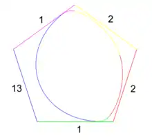
The cubic B-spline curve at the right is the same as the curve above and is now described in terms of knot intervals. If you remember, the curve has 10 knots in the knot vector. Discarding the n-1 knots on either end of the vector yields the 6 parameter values over which the B-spline curve is defined. 5 Bézier curves will span these parameter values, which just happens to be the number of sides on the control polygon. We can assign each side of the control polygon to a Bézier curve and the parameter interval over which the Bézier curve is defined. In the figure at right, the colors show which side corresponds to which curve. Let's talk about knot intervals a bit first before we talk about knot insertion.
Let's look at what the intervals tell us about the knot vector. If the interval for a curve is 1, the parameter values could go from [0,1], [2,3], or even [156,157]. It doesn't really matter what the values of the knot vectors are, since we know that only the intervals matter. In this way, we can arbitrarily construct a knot vector starting at any value. If we started at 0 and at the topmost control point, then the knot vector would be 2, 4, 5, 18, and 19, if we proceed in a clockwise manner. We must also take into account the end condition knots at either end of the vector. This is just another way of thinking about a B-spline curve. The intervals can be any number, including 0. What happens at a 0 interval? Well, if we had a 0, then that corresponds to a repeated knot. Hopefully, you are now thinking about the de Boor algorithm and wondering how we can get the Bézier curves that a periodic B-spline curve would generate.